Karhunen–Loève theorem
In the theory of stochastic processes, the Karhunen–Loève theorem (named after Kari Karhunen and Michel Loève) is a representation of a stochastic process as an infinite linear combination of orthogonal functions, analogous to a Fourier series representation of a function on a bounded interval. Stochastic processes given by infinite series of this form were considered earlier by Damodar Dharmananda Kosambi.[1] There exist many such expansions of a stochastic process: if the process is indexed over [a, b], any orthonormal basis of L2([a, b]) yields an expansion thereof in that form. The importance of the Karhunen–Loève theorem is that it yields the best such basis in the sense that it minimizes the total mean squared error.
In contrast to a Fourier series where the coefficients are real numbers and the expansion basis consists of sinusoidal functions (that is, sine and cosine functions), the coefficients in the Karhunen–Loève theorem are random variables and the expansion basis depends on the process. In fact, the orthogonal basis functions used in this representation are determined by the covariance function of the process. One can think that the Karhunen–Loève transform adapts to the process in order to produce the best possible basis for its expansion.
In the case of a centered stochastic process {Xt}t ∈ [a, b] (where centered means that the expectations E(Xt) are defined and equal to 0 for all values of the parameter t in [a, b]) satisfying a technical continuity condition, Xt admits a decomposition
where Zk are pairwise uncorrelated random variables and the functions ek are continuous real-valued functions on [a, b] that are pairwise orthogonal in L2[a, b]. It is therefore sometimes said that the expansion is bi-orthogonal since the random coefficients Zk are orthogonal in the probability space while the deterministic functions ek are orthogonal in the time domain. The general case of a process Xt that is not centered can be brought back to the case of a centered process by considering (Xt − E(Xt)) which is a centered process.
Moreover, if the process is Gaussian, then the random variables Zk are Gaussian and stochastically independent. This result generalizes the Karhunen–Loève transform. An important example of a centered real stochastic process on [0,1] is the Wiener process; the Karhunen–Loève theorem can be used to provide a canonical orthogonal representation for it. In this case the expansion consists of sinusoidal functions.
The above expansion into uncorrelated random variables is also known as the Karhunen–Loève expansion or Karhunen–Loève decomposition. The empirical version (i.e., with the coefficients computed from a sample) is known as the Karhunen–Loève transform (KLT), principal component analysis, proper orthogonal decomposition (POD), Empirical orthogonal functions (a term used in meteorology and geophysics), or the Hotelling transform.
Contents |
Formulation
- Throughout this article, we will consider a square integrable zero-mean random process Xt defined over a probability space (Ω,F,P) and indexed over a closed interval [a, b], with covariance function KX(s,t). We thus have:
![\forall t\in [a,b], X_t\in L^2(\Omega,\mathcal{F},\mathrm{P}),](/2012-wikipedia_en_all_nopic_01_2012/I/7a25aea55a02d3a94d14fba708784533.png)
![\forall t\in [a,b], \mathrm{E}[X_t]=0,](/2012-wikipedia_en_all_nopic_01_2012/I/8a9c13dee8d2708ec9bfa78f86397b11.png)
![\forall t,s \in [a,b], K_X(s,t)=\mathrm{E}[X_s X_t].](/2012-wikipedia_en_all_nopic_01_2012/I/05977f77813dc888245d1f09ddb208c3.png)
- We associate to KX a linear operator TKX defined in the following way:
![\begin{array}{rrl}
T_{K_X}: L^2([a,b]) &\rightarrow & L^2([a,b])\\
f(t) & \mapsto & \int_{[a,b]} K_X(s,t) f(s) ds
\end{array}](/2012-wikipedia_en_all_nopic_01_2012/I/893be05e2a362e75705e261b64b0da66.png)
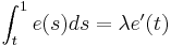
Since TKX is a linear operator, it makes sense to talk about its eigenvalues λk and eigenfunctions ek, which are found solving the homogeneous Fredholm integral equation of the second kind![\int_{[a,b]} K_X(s,t) e_k(s)\,ds=\lambda_k e_k(t)](/2012-wikipedia_en_all_nopic_01_2012/I/5de315ff8a1c00376b23b5da5ccaf7c8.png)
Statement of the theorem
Theorem. Let Xt be a zero-mean square integrable stochastic process defined over a probability space (Ω,F,P) and indexed over a closed and bounded interval [a, b], with continuous covariance function KX(s,t).
Then KX(s,t) is a Mercer kernel and letting ek be an orthonormal basis of L2([a, b]) formed by the eigenfunctions of TKX with respective eigenvalues λk, Xt admits the following representation
where the convergence is in L2, uniform in t and
Furthermore, the random variables Zk have zero-mean, are uncorrelated and have variance λk
![\mathrm{E}[Z_k]=0,~\forall k\in\mathbb{N} \quad\quad\mbox{and}\quad\quad \mathrm{E}[Z_i Z_j]=\delta_{ij} \lambda_j,~\forall i,j\in \mathbb{N}](/2012-wikipedia_en_all_nopic_01_2012/I/3a1a15680cc5f6ad8e1899fa932922f5.png)
Note that by generalizations of Mercer's theorem we can replace the interval [a, b] with other compact spaces C and the Lebesgue measure on [a, b] with a Borel measure whose support is C.
Proof
- The covariance function KX satisfies the definition of a Mercer kernel. By Mercer's theorem, there consequently exists a set {λk,ek(t)} of eigenvalues and eigenfunctions of TKX forming an orthonormal basis of L2([a,b]), and KX can be expressed as
- The process Xt can be expanded in terms of the eigenfunctions ek as:
where the coefficients (random variables) Zk are given by the projection of Xt on the respective eigenfunctions![Z_k=\int_{[a,b]} X_t e_k(t) \,dt](/2012-wikipedia_en_all_nopic_01_2012/I/e4b45abb1523f8da0c5e7b2a2eec40b4.png)
- We may then derive
![\mathrm{E}[Z_k]=\mathrm{E}\left[\int_{[a,b]} X_t e_k(t) \,dt\right]=\int_{[a,b]} \mathrm{E}[X_t] e_k(t) dt=0](/2012-wikipedia_en_all_nopic_01_2012/I/7250048e8500a6e0adb5f9c999e08107.png)
and:![\begin{array}[t]{rl}
\mathrm{E}[Z_i Z_j]&=\mathrm{E}\left[ \int_{[a,b]}\int_{[a,b]} X_t X_s e_j(t)e_i(s) dt\, ds\right]\\
&=\int_{[a,b]}\int_{[a,b]} \mathrm{E}\left[X_t X_s\right] e_j(t)e_i(s) dt\, ds\\
&=\int_{[a,b]}\int_{[a,b]} K_X(s,t) e_j(t)e_i(s) dt \, ds\\
&=\int_{[a,b]} e_i(s)\left(\int_{[a,b]} K_X(s,t) e_j(t) dt\right) ds\\
&=\lambda_j \int_{[a,b]} e_i(s) e_j(s) ds\\
&=\delta_{ij}\lambda_j
\end{array}](/2012-wikipedia_en_all_nopic_01_2012/I/78087461cd1159e541f90399e6d869d6.png)
where we have used the fact that the ek are eigenfunctions of TKX and are orthonormal.
- Let us now show that the convergence is in L2:
let .
.
![\begin{align}
\mathrm{E}[|X_t-S_N|^2]&=\mathrm{E}[X_t^2]%2B\mathrm{E}[S_N^2]-2\mathrm{E}[X_t S_N]\\
&=K_X(t,t)%2B\mathrm{E}\left[\sum_{k=1}^N \sum_{l=1}^N Z_k Z_l e_k(t)e_l(t) \right] -2\mathrm{E}\left[X_t\sum_{k=1}^N Z_k e_k(t)\right]\\
&=K_X(t,t)%2B\sum_{k=1}^N \lambda_k e_k(t)^2 -2\mathrm{E}\left[\sum_{k=1}^N \int_0^1 X_t X_s e_k(s) e_k(t) ds\right]\\
&=K_X(t,t)-\sum_{k=1}^N \lambda_k e_k(t)^2
\end{align}](/2012-wikipedia_en_all_nopic_01_2012/I/d09d9250e6ea9aa75de4b109c8261d70.png)
which goes to 0 by Mercer's theorem.
Properties of the Karhunen–Loève transform
Special case: Gaussian distribution
Since the limit in the mean of jointly Gaussian random variables is jointly Gaussian, and jointly Gaussian random (centered) variables are independent if and only if they are orthogonal, we can also conclude:
Theorem. The variables Zi have a joint Gaussian distribution and are stochastically independent if the original process {Xt}t is Gaussian.
In the gaussian case, since the variables Zi are independent, we can say more:
almost surely.
The Karhunen-Loève transform decorrelates the process
This is a consequence of the independence of the Zk.
The Karhunen-Loève expansion minimizes the total mean square error
In the introduction, we mentioned that the truncated Karhunen-Loeve expansion was the best approximation of the original process in the sense that it reduces the total mean-square error resulting of its truncation. Because of this property, it is often said that the KL transform optimally compacts the energy.
More specifically, given any orthonormal basis {fk} of L2([a, b]), we may decompose the process Xt as:
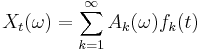
where ![A_k(\omega)=\int_{[a,b]} X_t(\omega) f_k(t)\,dt](/2012-wikipedia_en_all_nopic_01_2012/I/01b868afc90e5a4537fc35f986c21b1f.png)
and we may approximate Xt by the finite sum 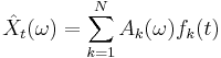 for some integer N.
Claim. Of all such approximations, the KL approximation is the one that minimizes the total mean square error (provided we have arranged the eigenvalues in decreasing order).
Consider the error resulting from the truncation at the N-th term in the following orthonormal expansion:
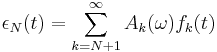
The mean-square error εN2(t) can be written as:
![\begin{align}
\varepsilon_N^2(t)&=\mathrm{E}\left[\sum_{i=N%2B1}^\infty \sum_{j=N%2B1}^\infty A_i(\omega) A_j(\omega) f_i(t) f_j(t)\right]\\
&=\sum_{i=N%2B1}^\infty \sum_{j=N%2B1}^\infty \mathrm{E}\left[\int_{[a, b]}\int_{[a, b]} X_t X_s f_i(t)f_j(s) ds\, dt\right] f_i(t) f_j(t)\\
&=\sum_{i=N%2B1}^\infty \sum_{j=N%2B1}^\infty f_i(t) f_j(t) \int_{[a, b]}\int_{[a, b]}K_X(s,t) f_i(t)f_j(s) ds\, dt
\end{align}](/2012-wikipedia_en_all_nopic_01_2012/I/f6a1fb62f169c0581b39177e1299e0af.png)
We then integrate this last equality over [a, b]. The orthonormality of the fk yields:
![\int_{[a, b]} \varepsilon_N^2(t) dt=\sum_{k=N%2B1}^\infty \int_{[a, b]}\int_{[a, b]} K_X(s,t) f_k(t)f_k(s) ds\, dt](/2012-wikipedia_en_all_nopic_01_2012/I/d34f97120a0cf73960ae98f0c9839f64.png)
The problem of minimizing the total mean-square error thus comes down to minimizing the right hand side of this equality subject to the constraint that the fk be normalized. We hence introduce βk, the Lagrangian multipliers associated with these constraints, and aim at minimizing the following function:
![Er[f_k(t),k\in\{N%2B1,\ldots\}]=\sum_{k=N%2B1}^\infty \int_{[a, b]}\int_{[a, b]} K_X(s,t) f_k(t)f_k(s) ds dt-\beta_k \left(\int_{[a, b]} f_k(t) f_k(t) dt -1\right)](/2012-wikipedia_en_all_nopic_01_2012/I/7367c21665a62a58a42944a1d806d087.png)
Differentiating with respect to fi(t)$ and setting the derivative to 0 yields:
![\frac{\partial Er}{\partial f_i(t)}=\int_{[a, b]} \left(\int_{[a, b]} K_X(s,t) f_i(s) ds -\beta_i f_i(t)\right)dt=0](/2012-wikipedia_en_all_nopic_01_2012/I/0dff5173fabdf40a6429936101022574.png)
which is satisfied in particular when ![\int_{[a, b]} K_X(s,t) f_i(s) \,ds =\beta_i f_i(t)](/2012-wikipedia_en_all_nopic_01_2012/I/dbd578e177a721c138f5ebdb25e1ee9d.png) , in other words when the fk are chosen to be the eigenfunctions of TKX, hence resulting in the KL expansion.
, in other words when the fk are chosen to be the eigenfunctions of TKX, hence resulting in the KL expansion.
Explained variance
An important observation is that since the random coefficients Zk of the KL expansion are uncorrelated, the Bienaymé formula asserts that the variance of Xt is simply the sum of the variances of the individual components of the sum:
![\begin{align}
\mbox{Var}[X_t]&=\sum_{k=0}^\infty e_k(t)^2 \mbox{Var}[Z_k]=\sum_{k=1}^\infty \lambda_k e_k(t)^2
\end{align}](/2012-wikipedia_en_all_nopic_01_2012/I/4b8094af98fbdd842a82681d56ee875a.png)
Integrating over [a, b] and using the orthonormality of the ek, we obtain that the total variance of the process is:
![\int_{[a,b]} \mbox{Var}[X_t] dt=\sum_{k=1}^\infty \lambda_k](/2012-wikipedia_en_all_nopic_01_2012/I/c41510b5c1dda73df557e5b4a1d63629.png)
In particular, the total variance of the N-truncated approximation is  . As a result, the N-truncated expansion explains
  of the variance; and if we are content with an approximation that explains, say, 95% of the variance, then we just have to determine an
  such that
 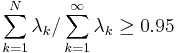 .
.
The Karhunen-Loève expansion has the minimum representation entropy property
Principal Component Analysis
We have established the Karhunen-Loève theorem and derived a few properties thereof. We also noted that one hurdle in its application was the numerical cost of determining the eigenvalues and eigenfunctions of its covariance operator through the Fredholm integral equation of the second kind .
However, when applied to a discrete and finite process  , the problem takes a much simpler form and standard algebra can be used to carry out the calculations.
Note that a continuous process can also be sampled at N points in time in order to reduce the problem to a finite version.
We henceforth consider a random N-dimensional vector  . As mentioned above, X could contain N samples of a signal but it can hold many more representations depending on the field of application. For instance it could be the answers to a survey or economic data in an econometrics analysis.
As in the continuous version, we assume that X is centered, otherwise we can let  (where
  is the mean vector of X) which is centered.
Let us adapt the procedure to the discrete case.
Covariance matrix
Recall that the main implication and difficulty of the KL transformation is computing the eigenvectors of the linear operator associated to the covariance function, which are given by the solutions to the integral equation written above.
Define Σ, the covariance matrix of X. Σ is an N by N matrix whose elements are given by:
![\Sigma_{ij}=E[X_i X_j],\qquad \forall i,j \in \{1,\ldots,N\}](/2012-wikipedia_en_all_nopic_01_2012/I/ffa6e321039ac24102a90cae9ad9c952.png)
Rewriting the above integral equation to suit the discrete case, we observe that it turns into:
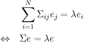
where  is an N-dimensional vector.
The integral equation thus reduces to a simple matrix eigenvalue problem, which explains why the PCA has such a broad domain of applications.
Since Σ is a positive definite symmetric matrix, it possesses a set of orthonormal eigenvectors forming a basis of  , and we write
  this set of eigenvalues and corresponding eigenvectors, listed in decreasing values of λi. Let also
  be the orthonormal matrix consisting of these eigenvectors:
Principal Component Transform
It remains to perform the actual KL transformation which we will call Principal Component Transform in this case. Recall that the transform was found by expanding the process with respect to the basis spanned by the eigenvectors of the covariance function. In this case, we hence have:
In a more compact form, the Principal Component Transform of X is defined by:
The i-th component of Y is  , the projection of X on
  and the inverse transform
  yields the expansion of
  on the space spanned by the :
As in the continuous case, we may reduce the dimensionality of the problem by truncating the sum at some  such that
  where α is the explained variance threshold we wish to set.
Examples
The Wiener process
There are numerous equivalent characterizations of the Wiener process which is a mathematical formalization of Brownian motion. Here we regard it as the centered standard Gaussian process Wt with covariance function

We restrict the time domain to [a,b]=[0,1] without loss of generality.
The eigenvectors of the covariance kernel are easily determined. These are
and the corresponding eigenvalues are
In order to find the eigenvalues and eigenvectors, we need to solve the integral equation:
![\begin{align}
\int_{[a,b]} K_W(s,t) e(s)ds&=\lambda e(t)\qquad \forall t, 0\leq t\leq 1\\
\int_0^1\min(s,t) e(s)ds&=\lambda e(t)\qquad \forall t, 0\leq t\leq 1 \\
\int_0^t s e(s) ds %2B t \int_t^1 e(s) ds &= \lambda e(t) \qquad \forall t, 0\leq t\leq 1
\end{align}](/2012-wikipedia_en_all_nopic_01_2012/I/1cb83603eb5169e62901cc000ea7abf3.png)
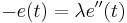
differentiating once with respect to t yields:
a second differentiation produces the following differential equation:
The general solution of which has the form:
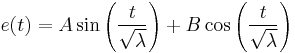
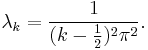
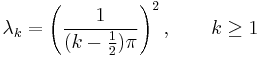
where A and B are two constants to be determined with the boundary conditions. Setting t=0 in the initial integral equation gives e(0)=0 which implies that B=0 and similarly, setting t=1 in the first differentiation yields e' (1)=0, whence:
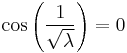
which in turn implies that eigenvalues of TKX are:
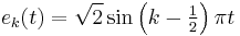
The corresponding eigenfunctions are thus of the form:
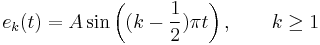
A is then chosen so as to normalize ek:
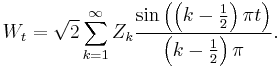
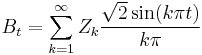
This gives the following representation of the Wiener process:
Theorem. There is a sequence {Zi}i of independent Gaussian random variables with mean zero and variance 1 such that
Note that this representation is only valid for ![t\in[0,1].](/2012-wikipedia_en_all_nopic_01_2012/I/de4ef1e33d30a0fa6fc661f8fed20bde.png) On larger intervals, the increments are not independent. As stated in the theorem, convergence is in the L2 norm and uniform in t.
On larger intervals, the increments are not independent. As stated in the theorem, convergence is in the L2 norm and uniform in t.
The Brownian bridge
Similarly the Brownian bridge  which is a stochastic process with covariance function
can be represented as the series
Applications
Adaptive optics systems sometimes use K–L functions to reconstruct wave-front phase information (Dai 1996, JOSA A).
Karhunen-Loève expansion is closely related to the Singular Value Decomposition. The latter has myriad applications in image processing, radar, seismology, and the like. If one has independent vector observations from a vector valued stochastic process then the left singular vectors are maximum likelihood estimates of the ensemble KL expansion.
See also
Notes
References
- Stark, Henry; Woods, John W. (1986). Probability, Random Processes, and Estimation Theory for Engineers. Prentice-Hall, Inc. ISBN 0-13-711706-X. http://openlibrary.org/books/OL21138080M/Probability_random_processes_and_estimation_theory_for_engineers.
- Ghanem, Roger; Spanos, Pol (1991). Stochastic finite elements: a spectral approach. Springer-Verlag. ISBN 0387974563. http://openlibrary.org/books/OL1865197M/Stochastic_finite_elements.
- Guikhman, I.; Skorokhod, A. (1977). Introduction a la Théorie des Processus Aléatoires. Éditions MIR.
- Simon, B. (1979). Functional Integration and Quantum Physics. Academic Press.
- Karhunen, Kari (1947). "Über lineare Methoden in der Wahrscheinlichkeitsrechnung". Ann. Acad. Sci. Fennicae. Ser. A. I. Math.-Phys. 37: 1–79.
- Loève, M. (1978). Probability theory. Vol. II, 4th ed.. Graduate Texts in Mathematics. 46. Springer-Verlag. ISBN 0-387-90262-7.
- Dai, G. (1996). "Modal wave-front reconstruction with Zernike polynomials and Karhunen–Loeve functions". JOSA A 13 (6): 1218. Bibcode 1996JOSAA..13.1218D. doi:10.1364/JOSAA.13.001218.
- Wu B., Zhu J., Najm F.(2005) "A Non-parametric Approach for Dynamic Range Estimation of Nonlinear Systems". In Proceedings of Design Automation Conference(841-844) 2005
- Wu B., Zhu J., Najm F.(2006) "Dynamic Range Estimation". IEEE Transactions on Computer-Aided Design of Integrated Circuits and Systems, Vol. 25 Issue:9 (1618-1636) 2006
- Jorgensen, Palle E. T.; Song, Myung-Sin (2007). "Entropy Encoding, Hilbert Space and Karhunen-Loeve Transforms". arXiv:math-ph/0701056. Bibcode 2007JMP....48j3503J.
- Mathar, Richard J. (2008). "Karhunen-Loeve basis functions of Kolmogorov turbulence in the sphere". Baltic Astronomy 17 (3/4): 383–398. Bibcode 2008BaltA..17..383M.
- Mathar, Richard J. (2009). "Modal decomposition of the von-Karman covariance of atmospheric turbulence in the circular entrance pupil". arXiv:0911.4710 [astro-ph.IM]. Bibcode 2009arXiv0911.4710M.
- Mathar, Richard J. (2010). "Karhunen-Loeve basis of Kolmogorov phase screens covering a rectangular stripe". Waves in Random and Complex Media 20 (1): 23–35. Bibcode 2020WRCM...20...23M. doi:10.1080/17455030903369677.
External links
- Mathematica KarhunenLoeveDecomposition function.
- E161: Computer Image Processing and Analysis notes by Pr. Ruye Wang at Harvey Mudd College [1]